Basic usage of edfinr

Introduction

The edfinr package provides tidy, analysis-ready school district finance data for the United States — NCES F-33 revenues and expenditures joined with enrollment, poverty, community, and labor-cost measures — assembled with an opinionated cleaning methodology. This vignette will help you get started with the package’s core functionality.

library(edfinr)
library(dplyr)
library(ggplot2)

Core function: get_finance_data()

The primary function in edfinr is get_finance_data(), which provides access to school finance data from school years 2011-12 through 2022-23. NCES F-33 data are released roughly two years after a fiscal year closes, so FY2023 (SY2022-23) is the most recent federal release. The function combines data from multiple sources:

Financial data: Revenue and expenditure data (including capital outlay, debt, and fund balances) from the National Center for Education Statistics (NCES) version of the F-33 survey.
Enrollment: Fall membership counts (F-33 item V33), the denominator for all per-pupil measures.
Demographics: Poverty estimates from the U.S. Census Bureau Small Area Income and Poverty Estimates (SAIPE).
Community characteristics: Income and education data from American Community Survey (ACS).
Labor costs: The NCES EDGE Comparable Wage Index for Teachers (CWIFT).
Inflation adjustments: Consumer Price Index for All Urban Consumers (CPI-U) data for constant dollar calculations.

Basic usage

The simplest way to use get_finance_data() is to specify a year and state. For example, to get finance data for Kentucky school districts from the 2022-23 school year:

ky_sy23 <- get_finance_data(yr = "2023", geo = "KY")
glimpse(ky_sy23)

## Rows: 171
## Columns: 59
## $ ncesid             <chr> "2100030", "2100070", "2100081", "2100090", "210012…
## $ year               <int> 2023, 2023, 2023, 2023, 2023, 2023, 2023, 2023, 202…
## $ state              <chr> "KY", "KY", "KY", "KY", "KY", "KY", "KY", "KY", "KY…
## $ dist_name          <chr> "Adair County", "Allen County", "Muhlenberg County"…
## $ enroll             <dbl> 2622, 3149, 4486, 405, 3752, 3261, 317, 1052, 692, …
## $ rev_total_pp       <dbl> 14490.85, 14258.18, 15921.53, 27017.28, 13804.90, 1…
## $ rev_local_pp       <dbl> 2803.204, 2772.626, 4959.206, 17746.180, 4358.475, …
## $ rev_state_pp       <dbl> 8819.222, 8033.344, 8473.696, 8560.875, 7578.625, 8…
## $ rev_fed_pp         <dbl> 2868.4211, 3452.2070, 2488.6313, 710.2285, 1867.803…
## $ rev_total          <dbl> 37995000, 44899000, 71424000, 10942000, 51796000, 5…
## $ rev_local          <dbl> 7350000, 8731000, 22247000, 7187203, 16353000, 1127…
## $ rev_state          <dbl> 23124000, 25297000, 38013000, 3467155, 28435000, 27…
## $ rev_fed            <dbl> 7521000.0, 10871000.0, 11164000.0, 287642.6, 700800…
## $ rev_total_unadj    <dbl> 38897000, 45331000, 73317000, 11348000, 52150000, 5…
## $ rev_local_unadj    <dbl> 7350000, 8731000, 22728000, 7446000, 16361000, 1127…
## $ rev_state_unadj    <dbl> 24026000, 25729000, 39425000, 3604000, 28781000, 28…
## $ rev_fed_unadj      <dbl> 7521000, 10871000, 11164000, 298000, 7008000, 12719…
## $ rev_state_unadj_pp <dbl> 9163.234, 8170.530, 8788.453, 8898.765, 7670.842, 8…
## $ rev_local_unadj_pp <dbl> 2803.204, 2772.626, 5066.429, 18385.185, 4360.608, …
## $ rev_state_cap_debt <dbl> 902000, 432000, 1412000, 12000, 346000, 545000, 299…
## $ exp_cur_pp         <dbl> 13545.00, 12352.49, 13648.24, 25486.42, 12208.16, 1…
## $ exp_cap_total_pp   <dbl> 954.6148, 742.4579, 1251.2260, 506.1728, 352.0789, …
## $ rev_exp_pp_diff    <dbl> 945.8429, 1905.6843, 2273.2947, 1530.8642, 1596.748…
## $ exp_cur_st_loc     <dbl> 30583000, 33757000, 44193000, 10001000, 36509000, 4…
## $ exp_cur_fed        <dbl> 4871000, 5142000, 15670000, 320000, 4970000, 769300…
## $ exp_cur_resa       <dbl> NA, NA, NA, NA, NA, NA, NA, NA, NA, NA, NA, NA, NA,…
## $ exp_cur_total      <dbl> 35515000, 38898000, 61226000, 10322000, 45805000, 4…
## $ exp_cap_total      <dbl> 2503000, 2338000, 5613000, 205000, 1321000, 1014000…
## $ cpi_sy12           <dbl> 1.316923, 1.316923, 1.316923, 1.316923, 1.316923, 1…
## $ mhi                <dbl> 50316, 59029, 52672, 209250, 71747, 54263, 44688, 6…
## $ mean_hhi           <dbl> 67346.51, 77189.80, 77400.74, 300224.55, 88198.54, …
## $ mpv                <dbl> 134800, 176300, 121300, 808100, 213200, 130300, 115…
## $ adult_pop          <dbl> 12806, 14649, 21925, 1547, 16682, 15469, 1120, 5512…
## $ ba_plus_pop        <dbl> 2402, 2546, 2844, 1219, 4290, 3819, 214, 1028, 486,…
## $ ba_plus_pct        <dbl> 0.1875683, 0.1738003, 0.1297149, 0.7879767, 0.25716…
## $ gini               <dbl> 0.4840, 0.4595, 0.4853, 0.5020, 0.4053, 0.4698, 0.4…
## $ owner_pct          <dbl> 0.7622388, 0.7674478, 0.8193851, 0.9395405, 0.77948…
## $ snap_pct           <dbl> 0.15702834, 0.13003057, 0.15020524, 0.01088271, 0.0…
## $ unemp_rate         <dbl> 0.07738380, 0.07532628, 0.04063083, 0.04275742, 0.0…
## $ total_pop          <dbl> 19264, 21788, 30568, 2581, 24613, 21580, 1378, 7582…
## $ student_pop        <dbl> 2862, 3702, 4726, 461, 4324, 3533, 220, 1153, 403, …
## $ stpov_pop          <dbl> 763, 790, 1189, 11, 487, 843, 47, 241, 143, 473, 92…
## $ stpov_pct          <dbl> 0.26659679, 0.21339816, 0.25158697, 0.02386117, 0.1…
## $ cong_dist          <int> 2101, 2101, 2101, 2103, 2106, 2104, 2104, 2101, 210…
## $ state_leaid        <chr> "KY-001001000", "KY-002005000", "KY-089445000", "KY…
## $ county             <chr> "Adair County", "Allen County", "Muhlenberg County"…
## $ cbsa               <chr> "N", "14540", "16420", "31140", "23180", "26580", "…
## $ urbanicity_raw     <int> 33, 41, 41, 21, 32, 13, 42, 43, 33, 32, 41, 42, 21,…
## $ urbanicity_raw_cat <fct> "Town, Remote", "Rural, Fringe", "Rural, Fringe", "…
## $ urbanicity         <fct> Town, Rural, Rural, Suburb, Town, City, Rural, Rura…
## $ land_area_sq_mi    <dbl> 405.292, 343.724, 467.280, 2.991, 202.260, 13.437, …
## $ s_per_sq_mi        <dbl> 6.469410, 9.161420, 9.600240, 135.406219, 18.550381…
## $ schlev             <chr> "03", "03", "03", "01", "03", "03", "03", "03", "03…
## $ lea_type           <fct> Regular public school district that is not a compon…
## $ lea_type_id        <int> 1, 1, 1, 1, 1, 1, 1, 1, 1, 1, 1, 1, 1, 1, 1, 1, 1, …
## $ osp_pct            <dbl> 0.0000000000, 0.0000000000, 0.0000000000, 0.0347197…
## $ c11_spike_flag     <lgl> FALSE, FALSE, FALSE, FALSE, FALSE, FALSE, FALSE, FA…
## $ cwift_est          <dbl> 0.705, 0.833, 0.829, 0.915, 0.804, 0.847, 0.733, 0.…
## $ cwift_imputed      <lgl> TRUE, TRUE, TRUE, TRUE, TRUE, TRUE, TRUE, TRUE, TRU…

Dataset types: skinny vs. full

By default, get_finance_data() returns a “skinny” dataset with 59 essential variables covering:

District identifiers and characteristics.
Total revenues by source (local, state, federal).
Current expenditures and total capital outlay (exp_cap_total, exp_cap_total_pp).
Key demographic and economic indicators (including the CWIFT teacher-wage index).
District land area and student density (land_area_sq_mi, s_per_sq_mi).

For more detailed analysis, you can request the “full” dataset with 124 variables that includes:

All skinny dataset variables.
Detailed expenditure data.
Data on spending of temporary pandemic-related federal funding.
Detailed capital outlay, debt stocks, and fund balances (see the “Capital and Facilities” article).
The CWIFT standard error and imputation method (see the “CWIFT” article).

ky_full_sy23 <- get_finance_data(yr = "2023", geo = "KY", dataset_type = "full")
setdiff(names(ky_full_sy23), names(ky_sy23))

##  [1] "exp_emp_salary"             "exp_emp_bene"              
##  [3] "exp_textbooks"              "exp_utilities"             
##  [5] "exp_tech_supp"              "exp_tech_equip"            
##  [7] "exp_pay_private_sch"        "exp_pay_charter_sch"       
##  [9] "exp_pay_other_lea"          "exp_other_sys_pay"         
## [11] "exp_instr_total"            "exp_instr_sal"             
## [13] "exp_instr_bene"             "exp_supp_stu_total"        
## [15] "exp_supp_stu_sal"           "exp_supp_stu_bene"         
## [17] "exp_supp_instr_total"       "exp_supp_instr_sal"        
## [19] "exp_supp_instr_bene"        "exp_supp_gen_admin_total"  
## [21] "exp_supp_gen_admin_sal"     "exp_supp_gen_admin_bene"   
## [23] "exp_supp_sch_admin_total"   "exp_supp_sch_admin_sal"    
## [25] "exp_supp_sch_admin_bene"    "exp_supp_ops_total"        
## [27] "exp_supp_ops_sal"           "exp_supp_ops_bene"         
## [29] "exp_supp_trans_total"       "exp_supp_trans_sal"        
## [31] "exp_supp_trans_bene"        "exp_central_serv_total"    
## [33] "exp_central_serv_sal"       "exp_central_serv_bene"     
## [35] "exp_noninstr_food_total"    "exp_noninstr_food_sal"     
## [37] "exp_noninstr_food_bene"     "exp_noninstr_ent_ops_total"
## [39] "exp_noninstr_ent_ops_bene"  "exp_noninstr_other"        
## [41] "exp_covid_total"            "exp_covid_instr"           
## [43] "exp_covid_supp"             "exp_covid_cap_out"         
## [45] "exp_covid_tech_supp"        "exp_covid_tech_equip"      
## [47] "exp_covid_supp_plant"       "exp_covid_food"            
## [49] "exp_cap_construction"       "exp_cap_land"              
## [51] "exp_cap_equip_instr"        "exp_cap_equip_other"       
## [53] "exp_cap_equip_nonspec"      "exp_debt_interest"         
## [55] "debt_lt_begin"              "debt_lt_issued"            
## [57] "debt_lt_retired"            "debt_lt_end"               
## [59] "debt_st_begin"              "debt_st_end"               
## [61] "fund_bal_debt_svc"          "fund_bal_bond"             
## [63] "fund_bal_other"             "cwift_se"                  
## [65] "cwift_impute_method"

Finding variables

With 124 variables in the full dataset, the data dictionary is the fastest way to find what you need. list_variables() returns it as a tibble, so you can filter and search it like any other data.

vars <- list_variables("full")
vars

## # A tibble: 124 × 7
##    name         type      category    source f33_item first_yr_avail description
##    <chr>        <chr>     <chr>       <chr>  <chr>    <chr>          <chr>      
##  1 ncesid       character id          NCES … LEAID    2012           NCES distr…
##  2 year         integer   time        NCES … YRDATA   2012           School yea…
##  3 state        character geographic  NCES … STATE    2012           State abbr…
##  4 dist_name    character id          NCES … NAME     2012           District n…
##  5 enroll       numeric   demographic NCES … V33      2012           Total dist…
##  6 rev_total_pp numeric   revenue     NCES … NA       2012           Total adju…
##  7 rev_local_pp numeric   revenue     NCES … NA       2012           Local adju…
##  8 rev_state_pp numeric   revenue     NCES … NA       2012           State adju…
##  9 rev_fed_pp   numeric   revenue     NCES … NA       2012           Federal ad…
## 10 rev_total    numeric   revenue     NCES … NA       2012           Total adju…
## # ℹ 114 more rows

# filter by category
list_variables("full", category = "debt")

## # A tibble: 9 × 7
##   name              type    category source  f33_item first_yr_avail description
##   <chr>             <chr>   <chr>    <chr>   <chr>    <chr>          <chr>      
## 1 debt_lt_begin     numeric debt     NCES F… _19H     2012           Long-term …
## 2 debt_lt_issued    numeric debt     NCES F… _21F     2012           Long-term …
## 3 debt_lt_retired   numeric debt     NCES F… _31F     2012           Long-term …
## 4 debt_lt_end       numeric debt     NCES F… _41F     2012           Long-term …
## 5 debt_st_begin     numeric debt     NCES F… _61V     2012           Short-term…
## 6 debt_st_end       numeric debt     NCES F… _66V     2012           Short-term…
## 7 fund_bal_debt_svc numeric debt     NCES F… W01      2012           Debt servi…
## 8 fund_bal_bond     numeric debt     NCES F… W31      2012           Bond fund …
## 9 fund_bal_other    numeric debt     NCES F… W61      2012           Other fund…

Multiple years and states

The get_finance_data() function makes it easy to access data across multiple years and states:

sec_data <- get_finance_data(
  yr = "2019:2023",  # years 2019 through 2023
  geo = "AL,AR,FL,GA,KY,LA,MS,MO,OK,SC,TN,TX"  # comma-separated state codes
)

us_sy23 <- get_finance_data(yr = "2023", geo = "all")

Downloads and caching

Only the requested year(s) are downloaded: each year is hosted as its own file (roughly 3-6 MB), so a single-year or short-range request is lightweight even though the full panel spans 2012-2023. Requesting yr = "all" downloads the entire history from one combined file.

Downloaded files are cached in R’s temporary directory for the length of your R session, so repeated calls with the same years re-read the cache instead of re-downloading. Two arguments control this behavior: refresh = TRUE forces a fresh download (for example, after a data update is announced), and quiet = TRUE suppresses the download progress messages.

# re-download even if a cached copy exists, without progress messages
ky_fresh <- get_finance_data(yr = "2023", geo = "KY", refresh = TRUE, quiet = TRUE)

Working with the data

Once you’ve retrieved the data, you can use standard data manipulation tools to analyze it. Here are some common analysis patterns:

ct_sy23 <- get_finance_data(yr = "2023", geo = "CT")

ggplot(ct_sy23) +
  geom_point(aes(
    x = rev_local / rev_total,
    y = rev_total_pp,
    color = urbanicity,
    size = enroll),
    alpha = .6) +
  scale_size_area(
    max_size = 10,
    labels = scales::label_comma()
    ) +
  scale_x_continuous(labels = scales::label_percent()) +
  scale_y_continuous(labels = scales::label_dollar()) +
  labs(
    title = "Connecticut Districts' Local Revenue Share vs. Total Revenue Per-Pupil, SY2022-23",
    x = "Local Share of Total Revenue",
    y = "Total Revenue Per-Pupil",
    size = "Enrollment",
    color = "Urbanicity") +
  theme_bw()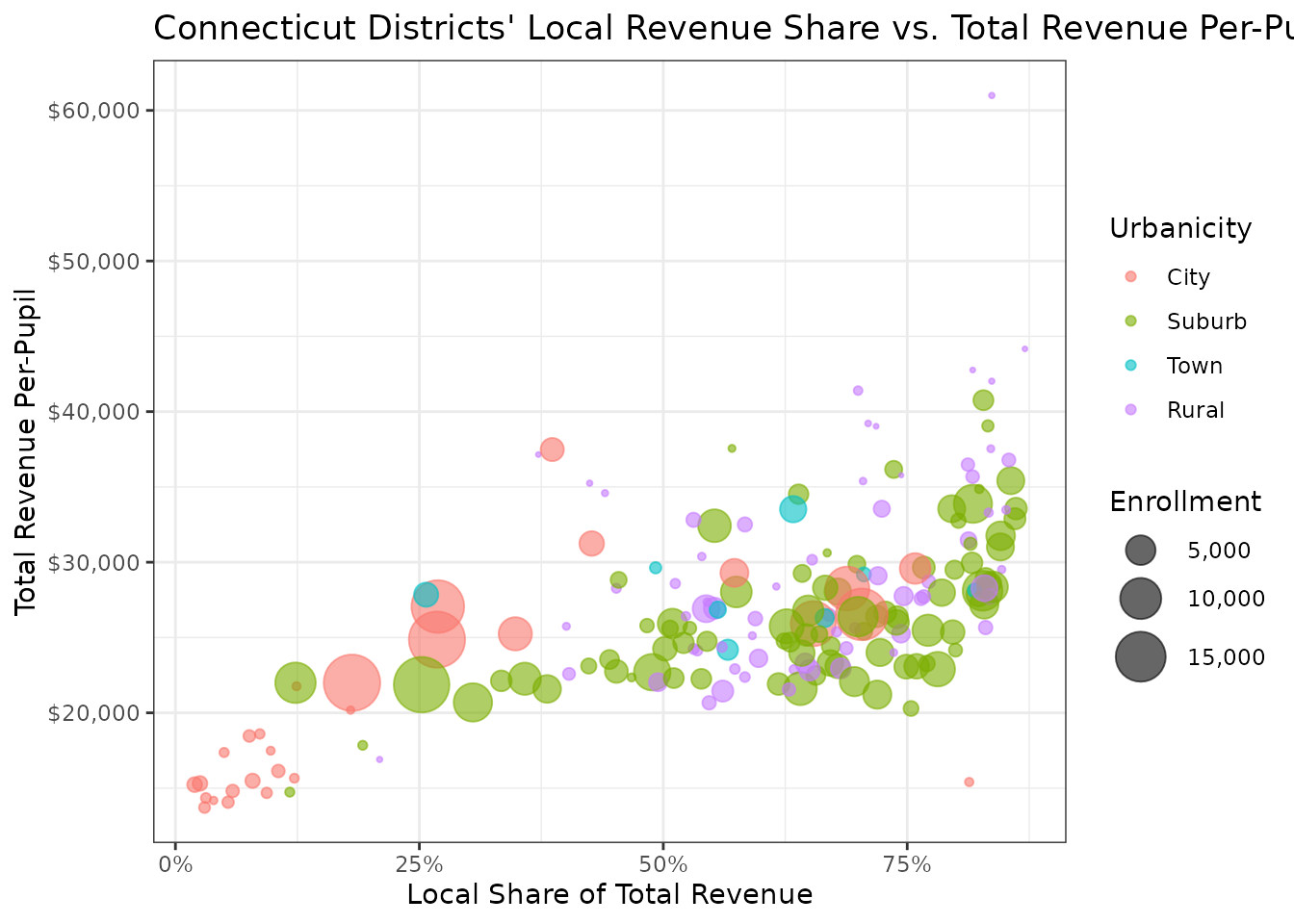

Scatterplot of Connecticut districts' local share of revenue versus total revenue per-pupil for SY2022-23, with point size showing enrollment and color showing urbanicity; the most locally-reliant districts tend to have higher total revenue per-pupil.

How do revenue sources differ by urbanicity?

# compare revenue mix across urbanicity groups (dollar-weighted)
revenue_analysis <- ct_sy23 |>
  group_by(urbanicity) |>
  summarize(
    pct_local = sum(rev_local, na.rm = TRUE) / sum(rev_total, na.rm = TRUE),
    pct_state = sum(rev_state, na.rm = TRUE) / sum(rev_total, na.rm = TRUE),
    pct_federal = sum(rev_fed, na.rm = TRUE) / sum(rev_total, na.rm = TRUE),
    n_districts = n(),
    enrollment = sum(enroll, na.rm = TRUE)
  )

revenue_analysis

## # A tibble: 4 × 6
##   urbanicity pct_local pct_state pct_federal n_districts enrollment
##   <fct>          <dbl>     <dbl>       <dbl>       <int>      <dbl>
## 1 City           0.434     0.442      0.124           29     127596
## 2 Suburb         0.644     0.289      0.0675          85     288189
## 3 Town           0.553     0.361      0.0859           8      14999
## 4 Rural          0.671     0.282      0.0476          65      53056