
Introduction
School finance data are messy in ways that summary statistics hide:
districts and states might change how they report revenues and
expenditures. Meanwhile, the set of districts in the panel shifts over
time. edfinr ships several diagnostic variables that make
these issues visible, and this article shows how to use them.
The examples below use the full national panel:
us <- get_finance_data(yr = "all", geo = "all", dataset_type = "skinny")
NA is not zero
Some F-33 items were originally coded -1 or
-2 to indicate missing values; edfinr recodes
these to NA during processing. An NA therefore
means the item was not reported, not that the district
spent or received nothing. Dropping NAs silently (for
example, with na.rm = TRUE in a ranking) keeps
incompletely-reporting districts in your analysis with partial values,
which can be worse than excluding them; decide explicitly.
Under version 0.2.0 (and beyond), edfinr also detects a
second F-33 missingness convention: some items are
zero-filled when missing, with a companion data-item
flag (FL_* = "M") marking them unreported. The data
processing proceture converts these flagged zero-fills to
NA for the COVID (exp_covid_*),
capital-detail, debt, fund-balance, CE fund-type, and expenditure-detail
items. The largest effect is on the COVID columns: all of New York
(including NYC) in every year and roughly a third to half of California
districts from FY2021 onward never reported them, and those districts
previously appeared as spending exactly $0. Genuine reported zeros are
preserved. Missingness also propagates through derived
measures rather than being treated as zero.
The state-revenue adjustment and c11_spike_flag
Following the EdBuild methodology, edfinr nets capital
and debt-related state aid (F-33 item C11) out of
rev_state, so that rev_state approximates
operating support. The pre-adjustment values are preserved in
rev_state_unadj and rev_state_unadj_pp, and
the netted-out C11 amount itself ships as
rev_state_cap_debt (in both datasets), so the adjustment
can be reconstructed directly:
rev_state_unadj - rev_state_cap_debt - rev_state equals the
state share of the other-system-payment adjustment. Because
rev_state_cap_debt feeds the adjustment arithmetic, it is
zero-filled, not NA, where districts did not report.
In a small number of district-years, the C11 adjustment produces an
anomalous spike – typically when a large one-time capital grant flows
through – and c11_spike_flag marks them:
## # A tibble: 12 × 2
##     year flagged
##    <int>   <int>
##  1  2012      58
##  2  2013      54
##  3  2014      47
##  4  2015      49
##  5  2016      42
##  6  2017      34
##  7  2018      24
##  8  2019      26
##  9  2020      37
## 10  2021      44
## 11  2022      23
## 12  2023      36
# which states account for the most flagged district-years?
us |>
  filter(c11_spike_flag) |>
  count(state, sort = TRUE) |>
  head(10)
## # A tibble: 10 × 2
## state n
## <chr> <int>
## 1 MA 105
## 2 CO 102
## 3 CA 68
## 4 PA 60
## 5 WY 32
## 6 IL 22
## 7 CT 17
## 8 GA 14
## 9 NJ 10
## 10 AK 7For a flagged district, the adjusted state-revenue series can dip or jump in ways the unadjusted series does not. Comparing the two makes the artifact obvious. Here we pick the largest district with multiple flagged years:
example_id <- us |>
  filter(c11_spike_flag) |>
  count(ncesid, wt = enroll, sort = TRUE) |>
  slice(1) |>
  pull(ncesid)

us |>
  filter(ncesid == example_id) |>
  select(year, dist_name, c11_spike_flag, rev_state_pp, rev_state_unadj_pp) |>
  pivot_longer(
    cols = c(rev_state_pp, rev_state_unadj_pp),
    names_to = "series", values_to = "value"
  ) |>
  mutate(series = ifelse(
    series == "rev_state_pp", "Adjusted (rev_state_pp)", "Unadjusted (rev_state_unadj_pp)"
  )) |>
  ggplot(aes(x = year, y = value, color = series)) +
  geom_line() +
  geom_point(aes(shape = c11_spike_flag), size = 2.5) +
  scale_x_continuous(breaks = seq(2013, 2023, 2)) +
  scale_y_continuous(labels = scales::label_dollar()) +
  scale_shape_manual(values = c(`FALSE` = 16, `TRUE` = 17)) +
  labs(
    title = "Adjusted vs. Unadjusted State Revenue Per-Pupil",
    subtitle = "Triangles mark years where c11_spike_flag is TRUE",
    x = "Year", y = "State Revenue Per-Pupil",
    color = NULL, shape = "Flagged"
  ) +
  theme_minimal()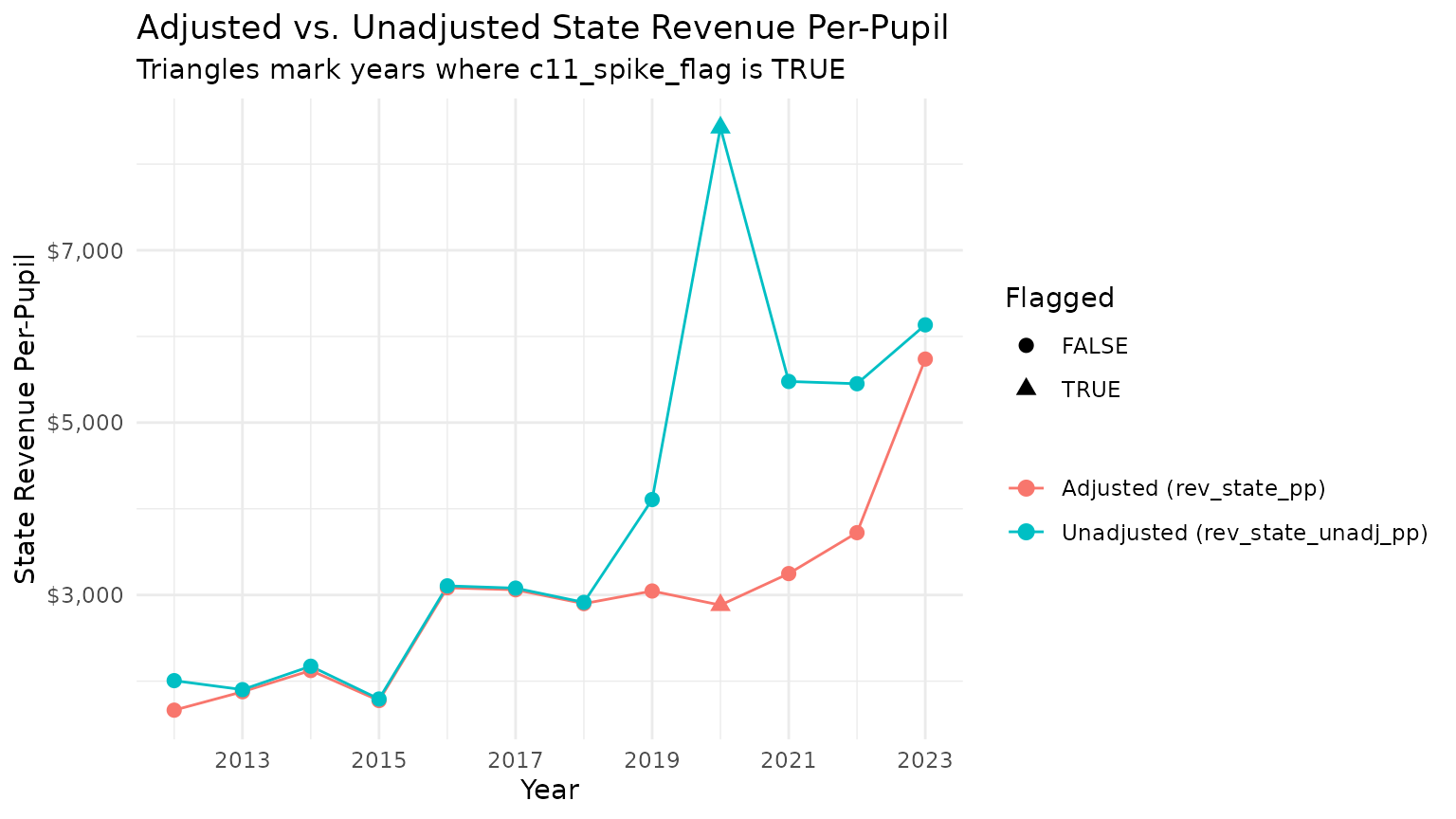
When analyzing state revenue over time, check
c11_spike_flag for your districts of interest, inspect
rev_state_cap_debt to see how large the adjustment actually
is, and consider using rev_state_unadj_pp (or excluding
flagged years) where the adjustment dominates the series.
Pass-through districts and osp_pct
Some districts pass a large share of the revenue they receive on to
other school systems (charter schools, other LEAs, private placements).
edfinr proportionally subtracts these payments from
revenues, and osp_pct reports the share of unadjusted total
revenue paid to other systems, so you can see how much the adjustment
matters for any district:
us_2023 <- us |> filter(year == 2023)

# how common are large pass-through shares?
us_2023 |>
  summarize(
    n = sum(!is.na(osp_pct)),
    over_10_pct = sum(osp_pct > 0.10, na.rm = TRUE),
    over_25_pct = sum(osp_pct > 0.25, na.rm = TRUE)
  )
## # A tibble: 1 × 3
## n over_10_pct over_25_pct
## <int> <int> <int>
## 1 16613 1028 230
# the largest pass-through districts, among districts with 1,000+ students
us_2023 |>
  filter(enroll >= 1000) |>
  arrange(desc(osp_pct)) |>
  select(dist_name, state, enroll, osp_pct, rev_total_pp) |>
  head(10)
## # A tibble: 10 × 5
## dist_name state enroll osp_pct rev_total_pp
## <chr> <chr> <dbl> <dbl> <dbl>
## 1 Orleans Parish LA 2040 0.760 85246.
## 2 Mitchell Sd 55 OR 1027 0.718 3731.
## 3 Mount Pleasant Elementary CA 1648 0.697 14303.
## 4 Santiam Canyon Sd 129j OR 2617 0.637 5244.
## 5 Prairie City Sd 4 OR 1089 0.532 6754.
## 6 Taconic And Green Regional School District… VT 1643 0.521 10670.
## 7 Grandview R-Ii MO 2387 0.500 5146.
## 8 Scio Sd 95 OR 1688 0.489 7826.
## 9 Chester-Upland Sd PA 3100 0.487 24554.
## 10 Sturgeon R-V MO 1445 0.483 5108.For high-osp_pct districts, per-pupil figures describe
the students the district serves directly, after the pass-through
dollars are removed. If you are more interested in every dollars a
district handles, use the rev_*_unadj variables
instead.
Panel composition: districts enter and exit
The universe of districts in edfinr is not constant
across years. The largest single discontinuity is in California:
beginning in school year 2018-19, a wave of California charter schools
switched to independent reporting and were assigned their own NCES LEA
IDs for the first time. Once in the NCES LEA universe, those new
charter-LEAs automatically show up in the F-33 finance survey. The
result is a jump in California district counts from 2019 onward that
reflects reporting structure, not new schools:
us |>
  mutate(group = ifelse(state == "CA", "California", "All other states")) |>
  count(group, year) |>
  ggplot(aes(x = year, y = n)) +
  geom_line() +
  geom_point(size = 1) +
  facet_wrap(~group, scales = "free_y") +
  scale_x_continuous(breaks = seq(2013, 2023, 2)) +
  labs(
    title = "Districts in the edfinr Panel by Year",
    subtitle = "The 2019 jump in California reflects charter schools becoming separate LEAs",
    x = "Year", y = "Districts"
  ) +
  theme_minimal()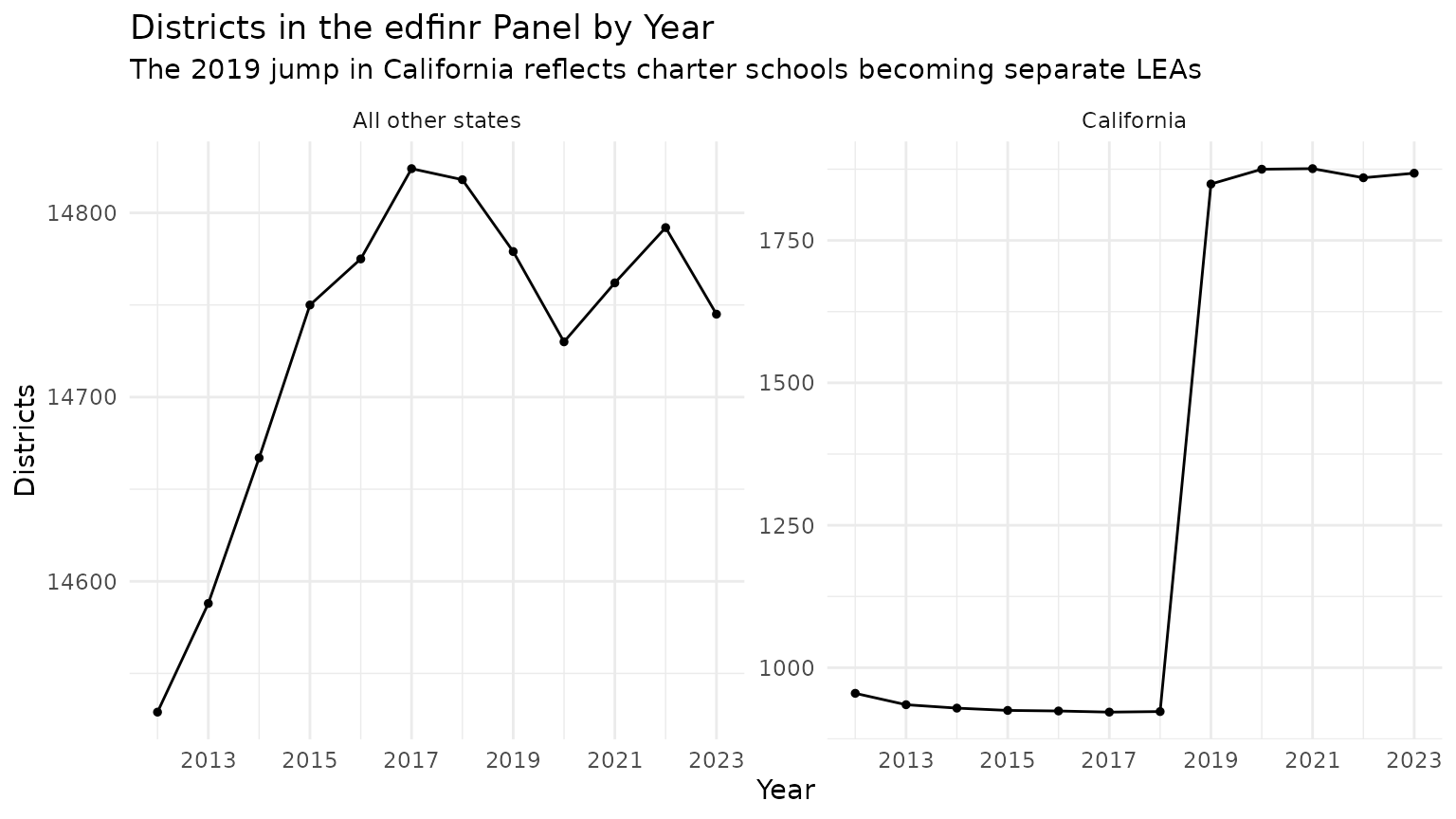
For longitudinal work, consider a consistent sample: keep only districts present in every year of your window.
Variable availability by year
Not every variable spans the full 2012-2023 panel. The data
dictionary’s first_yr_avail column records when each
variable enters the edfinr dataset:
list_variables("full") |>
  filter(first_yr_avail != "2012") |>
  select(name, first_yr_avail, description) |>
  arrange(first_yr_avail, name) |>
knitr::kable()| name | first_yr_avail | description |
|---|---|---|
| cwift_est | 2015 | Comparable Wage Index for Teachers estimate (LEA_CWIFTEST) |
| cwift_impute_method | 2015 | CWIFT imputation method: observed / interpolated_2019_2021 / carried_forward_2022 |
| cwift_imputed | 2015 | TRUE if the CWIFT value is imputed (interpolated or carried forward) |
| cwift_se | 2015 | Standard error of the CWIFT estimate (approximate for interpolated years) |
| exp_tech_equip | 2015 | Technology-related equipment (K14) |
| exp_tech_supp | 2015 | Technology-related supplies and purchased services (V02) |
| exp_utilities | 2015 | Utilities and energy services (V95) |
| exp_cur_fed | 2016 | Current expenditure from federal sources (ESSA item CE2; NA where the state did not report the fund-type split) |
| exp_cur_st_loc | 2016 | Current expenditure from state/local sources (ESSA item CE1; NA where the state did not report the fund-type split) |
| exp_cur_resa | 2018 | Current expenditure by RESA on behalf of LEAs (ESSA item CE3; NA where the state did not report the fund-type split) |
| exp_covid_cap_out | 2020 | COVID-19 Federal Assistance Funds - Capital outlay expenditures (AE4) |
| exp_covid_instr | 2020 | COVID-19 Federal Assistance Funds - Instructional expenditures (AE2) |
| exp_covid_supp | 2020 | COVID-19 Federal Assistance Funds - Support services expenditures (AE3) |
| exp_covid_tech_equip | 2020 | COVID-19 Federal Assistance Funds - Technology-related equipment expenditures (AE6) |
| exp_covid_tech_supp | 2020 | COVID-19 Federal Assistance Funds - Technology-related supplies and purchased services expenditures (AE5) |
| exp_covid_total | 2020 | COVID-19 Federal Assistance Funds - Total expenditures (AE1); NA where districts did not report the COVID items (all of NY in every year; roughly a third to half of CA districts from FY21) |
| exp_covid_food | 2021 | COVID-19 Federal Assistance Funds - Food services operations (AE8) |
| exp_covid_supp_plant | 2021 | COVID-19 Federal Assistance Funds - Support services operation and maintenance of plant expenditures (AE7) |
A multi-year average or trend that crosses one of these boundaries will mix real change with a coverage change.
first_yr_avail marks when a variable enters the
panel, but it does not capture partial coverage within years
where the variable is otherwise available. The Census Gazetteer fields
are a good example: land_area_sq_mi and
s_per_sq_mi both show
first_yr_avail == "2012", since they are populated from the
first year of the panel onward, but coverage is not uniform. Districts
without a Census boundary – charters, education service agencies, and
state-operated agencies – are always NA for these fields,
in every year, by design rather than by omission. And Vermont’s
FY2016-FY2021 Act 46 district consolidation left many post-consolidation
LEAs without a matching Gazetteer boundary, dropping match rates there
to roughly 7-12% for those years versus 97%+ elsewhere; restrict Vermont
trend analyses using these fields to FY2012-FY2015 or FY2022 onward.
Nothing in first_yr_avail flags this gap, so check a
variable’s actual non-missing rate by year and geography before assuming
uniform coverage.
Urbanicity: condensed vs. raw locale codes
The urbanicity factor condenses the NCES urban-centric
locale codes into four categories (City, Suburb, Town, Rural). The raw
12-category codes are also available as urbanicity_raw
(numeric) and urbanicity_raw_cat (labeled factor):
## # A tibble: 12 × 3
##    urbanicity_raw_cat urbanicity     n
##    <fct>              <fct>      <int>
##  1 City, Large        City        1707
##  2 City, Midsize      City         458
##  3 City, Small        City         656
##  4 Suburb, Large      Suburb      3249
##  5 Suburb, Midsize    Suburb       423
##  6 Suburb, Small      Suburb       292
##  7 Town, Fringe       Town         550
##  8 Town, Distant      Town        1190
##  9 Town, Remote       Town         789
## 10 Rural, Fringe      Rural       1925
## 11 Rural, Distant     Rural       3078
## 12 Rural, Remote      Rural       2296
The condensed categories are right for most summaries, but the raw codes can be helpful when the distinction within a category matters. For example, “Rural: Fringe” districts sit at metro edges and often look more like suburbs than like “Rural: Remote” districts.
Comparability checklist
Before publishing numbers built on edfinr data:
-
Check missingness for your variables and years;
decide explicitly how to treat
NAdistrict-years rather than relying onna.rm = TRUE. -
Check
first_yr_availfor every variable in a multi-year analysis, and remember it does not capture partial coverage (e.g., Vermont’s Gazetteer gap, FY2016-FY2021). -
Check
c11_spike_flag(and compare againstrev_state_unadj_pp) when state revenue is central to the analysis. -
Check
osp_pctwhen high-pass-through districts could distort per-pupil comparisons. - Use a consistent sample (or justify not doing so) for trend analyses, especially any that include California.
- Use CPI adjustment for any multi-year dollar comparison (see the “CPI Adjustments” vignette), and remember debt and fund-balance stocks stay nominal.