Community and Economic Context

Introduction

The communities that fund and attend public schools are deeply connected to school finance. Alongside the F-33 finance items, edfinr joins each district to community measures from the American Community Survey (ACS) 5-Year Estimates, poverty estimates from the Census Bureau’s Small Area Income and Poverty Estimates (SAIPE), and district land area from the Census Bureau’s Gazetteer Files. This article explores those variables and shows how to use them for a typical analysis task: comparing districts’ fiscal capacity (what a community can raise) with student need.

library(edfinr)
library(dplyr)
library(tidyr)
library(ggplot2)

The community variables

All of these are in the skinny dataset. The dictionary lists them with their source table codes:

list_variables("skinny") |>
  filter(source %in% c("5-Year ACS Survey", "Census Bureau SAIPE", "Census Bureau Gazetteer")) |>
  select(name, source, description) |>
  knitr::kable()

name	source	description
mhi	5-Year ACS Survey	Median household income (B19013_001)
mean_hhi	5-Year ACS Survey	Mean household income (aggregate household income / households)
mpv	5-Year ACS Survey	Median property value (B25077_001)
adult_pop	5-Year ACS Survey	Adult population (B15003_001)
ba_plus_pop	5-Year ACS Survey	Adults with bachelor’s degree or higher (B15003_022 + B15003_023 + B15003_024 + B15003_025)
ba_plus_pct	5-Year ACS Survey	Percent of adults with bachelor’s degree or higher
gini	5-Year ACS Survey	Gini index of income inequality (B19083_001)
owner_pct	5-Year ACS Survey	Owner-occupied share of occupied housing (B25003_002 / B25003_001)
snap_pct	5-Year ACS Survey	Share of households receiving SNAP (B22003_002 / B22003_001)
unemp_rate	5-Year ACS Survey	Unemployment rate (B23025_005 / B23025_003)
total_pop	Census Bureau SAIPE	Total population
student_pop	Census Bureau SAIPE	Student-aged population (5-17)
stpov_pop	Census Bureau SAIPE	Student-aged population in poverty
stpov_pct	Census Bureau SAIPE	Percent of students in poverty
land_area_sq_mi	Census Bureau Gazetteer	District land area in square miles (Gazetteer ALAND_SQMI; land only); NA for LEAs without a Census boundary (charters, ESAs, state-operated agencies)
s_per_sq_mi	Census Bureau Gazetteer	Students per square mile (enroll / land_area_sq_mi); NA, never Inf, where land area is zero or unavailable

Two timing caveats before using them:

1. ACS values are 5-year averages. The ACS estimates attached to a fiscal year summarize a five-year window, so they move slowly and lag sharp local changes (a plant closing, a housing boom). SAIPE poverty estimates are annual.
2. Estimates carry sampling error. ACS district-level estimates, especially for small districts, have nontrivial margins of error that edfinr does not carry. Treat small-district differences in gini, snap_pct, or unemp_rate as noisy.
3. SAIPE counts resident children, not enrolled students. stpov_pct measures poverty among children ages 5-17 who live within the district’s boundaries. Where many resident children attend charter, private, or neighboring schools – or where a charter LEA has no meaningful residential geography – the resident and enrolled populations can differ substantially.

The examples below use the most recent year:

us_2023 <- get_finance_data(yr = "2023", geo = "all")

Median vs. mean household income

mhi (median) and mean_hhi (mean) are different measures of community income. The mean is pulled upward by high-income households, so the mean-to-median ratio is a quick screen for skewed income distributions. This can be useful for identifying communities where a small wealthy population skews the mean income above the median income:

us_2023 |>
  filter(!is.na(mhi), !is.na(mean_hhi), mhi > 0) |>
  mutate(mean_to_median = mean_hhi / mhi) |>
  filter(enroll >= 1000) |>
  arrange(desc(mean_to_median)) |>
  select(dist_name, state, enroll, mhi, mean_hhi, mean_to_median) |>
  head(10)

## # A tibble: 10 × 6
##    dist_name                         state enroll    mhi mean_hhi mean_to_median
##    <chr>                             <chr>  <dbl>  <dbl>    <dbl>          <dbl>
##  1 Scarsdale Union Free School Dist… NY      4704 250001  606286.           2.43
##  2 Somerset Independent              KY      1615  34754   83973.           2.42
##  3 Aspen School District No. 1 In T… CO      1572  97015  216770.           2.23
##  4 West Lafayette Com School Corp    IN      2420  30111   66545.           2.21
##  5 Woodville Isd                     TX      1239  47886  103670.           2.16
##  6 Hillsborough City Elementary      CA      1294 250001  523236.           2.09
##  7 Dyersburg                         TN      2613  51846  104847.           2.02
##  8 Bronxville Union Free School Dis… NY      1555 215726  432323.           2.00
##  9 Boling Isd                        TX      1146  71797  143800.           2.00
## 10 Beverly Hills Unified             CA      3140 127472  250316.           1.96

Fiscal capacity: property wealth and local revenue

Local revenue depends heavily on the property tax base. Plotting per-pupil local revenue against median property value shows the relationship between the proxy for local fiscal capacity (MPV) and actual local revenue.

One caution before leaning on mpv as a capacity measure: it is the ACS median value of owner-occupied homes, a proxy for residential property wealth only. Formal fiscal-capacity measures use assessed (or equalized) valuation per pupil, which also counts commercial, industrial, and utility property and is scaled by enrollment. If your state publishes assessed valuation per pupil, use it; mpv is a nationally consistent fallback.

us_2023 |>
  filter(!is.na(mpv), !is.na(rev_local_pp), mpv > 0, rev_local_pp > 0,
         !is.na(urbanicity)) |>
  ggplot(aes(x = mpv, y = rev_local_pp, size = enroll, color = urbanicity)) +
  geom_point(alpha = 0.2) +
  geom_smooth(se = FALSE) +
  scale_x_log10(labels = scales::label_dollar()) +
  scale_y_continuous(labels = scales::label_dollar()) +
  scale_size_area(max_size = 10) +
  labs(
    title = "Local Revenue Tracks Property Wealth, SY2022-23",
    subtitle = "Each point is a district; log 10 scale x-axis",
    x = "Median Property Value (Log 10 scale)",
    y = "Local Revenue Per-Pupil",
    color = "Urbanicity",
    size = "Enrollment"
  ) +
  theme_minimal()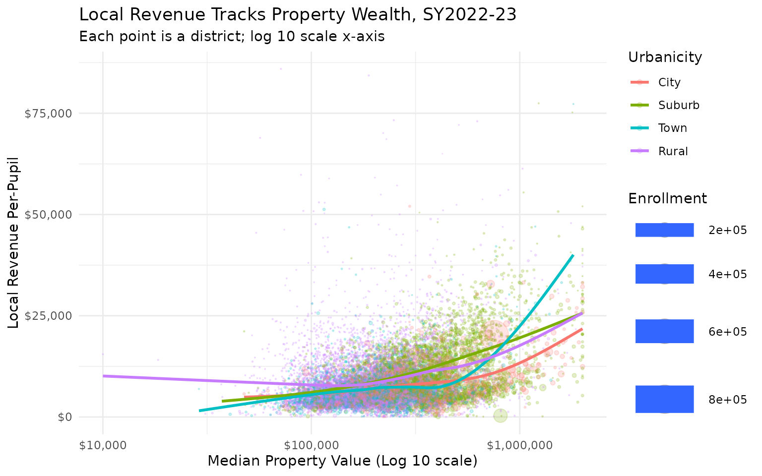

Student need: poverty and total revenue

The SAIPE-based stpov_pct measures the share of school-aged children in poverty. Whether total revenue rises with poverty – that is, whether state and federal aid more than offset weaker local capacity – varies sharply by state. Here is the national picture:

us_2023 |>
  filter(!is.na(stpov_pct), !is.na(rev_total_pp)) |>
  ggplot(aes(x = stpov_pct, y = rev_total_pp, size = enroll)) +
  geom_point(alpha = 0.15, size = 0.8) +
  geom_smooth(se = FALSE) +
  scale_x_continuous(labels = scales::label_percent()) +
  scale_y_continuous(labels = scales::label_dollar()) +
  scale_size_area(max_size = 10) +
  labs(
    title = "Student Poverty and Total Revenue Per-Pupil, SY2022-23",
    x = "Students in Poverty",
    y = "Total Revenue Per-Pupil",
    size = "Enrollment"
  ) +
  theme_minimal()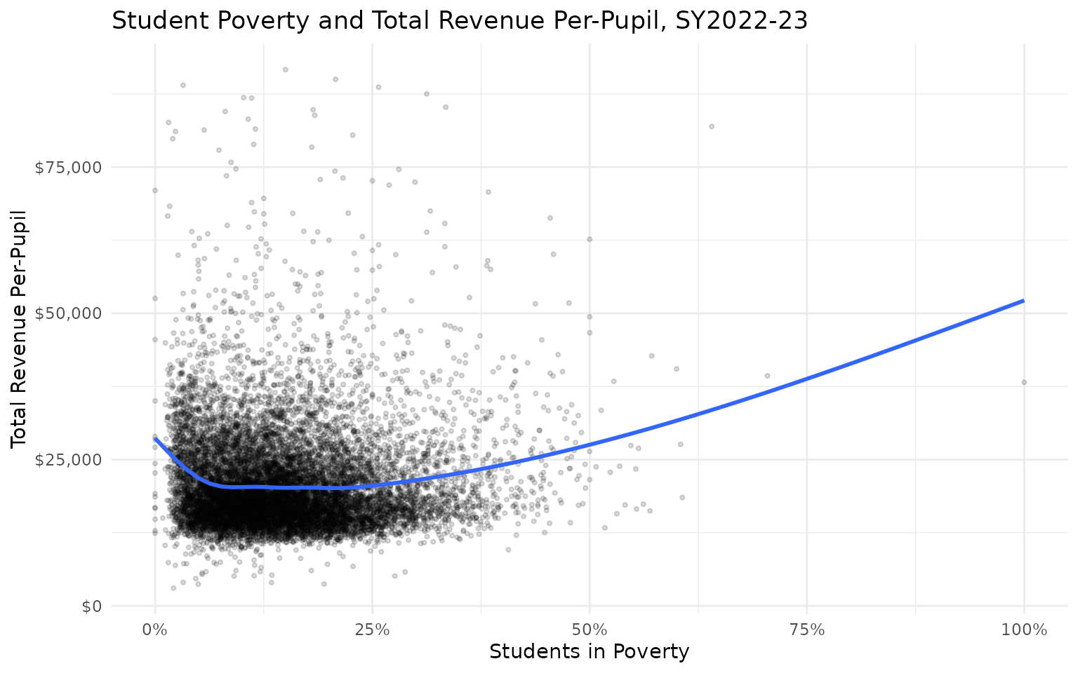

The national trend masks significant variation at the state level. It also compares nominal dollars: high-poverty urban districts sit disproportionately in high-wage labor markets, so a dollar buys less there than in a low-cost rural district. Cost-adjusted, within-state analyses can and do reach different conclusions than this raw national scatter. See the “CWIFT” article for the labor-cost adjustment.

Other indicators

gini (income inequality), owner_pct (owner-occupied housing), snap_pct (SNAP receipt), and unemp_rate (unemployment) round out the community picture. They are most useful as controls or descriptive context; their distributions differ enough across urbanicity to be worth checking before pooling:

us_2023 |>
  filter(!is.na(urbanicity)) |>
  select(urbanicity, gini, owner_pct, snap_pct, unemp_rate) |>
  pivot_longer(-urbanicity, names_to = "indicator", values_to = "value") |>
  filter(!is.na(value)) |>
  ggplot(aes(x = urbanicity, y = value)) +
  geom_boxplot(outlier.alpha = 0.1) +
  facet_wrap(~indicator, scales = "free_y") +
  labs(
    title = "Community Indicators by Urbanicity, SY2022-23",
    x = "Urbanicity", y = NULL
  ) +
  theme_minimal()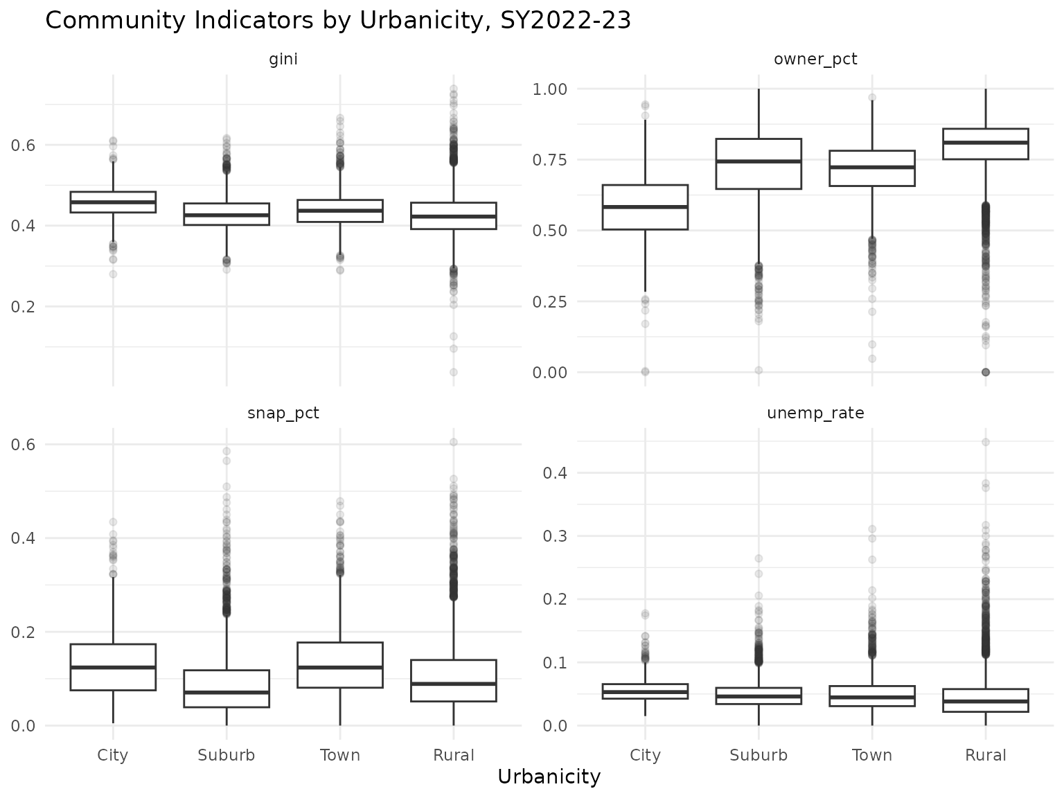

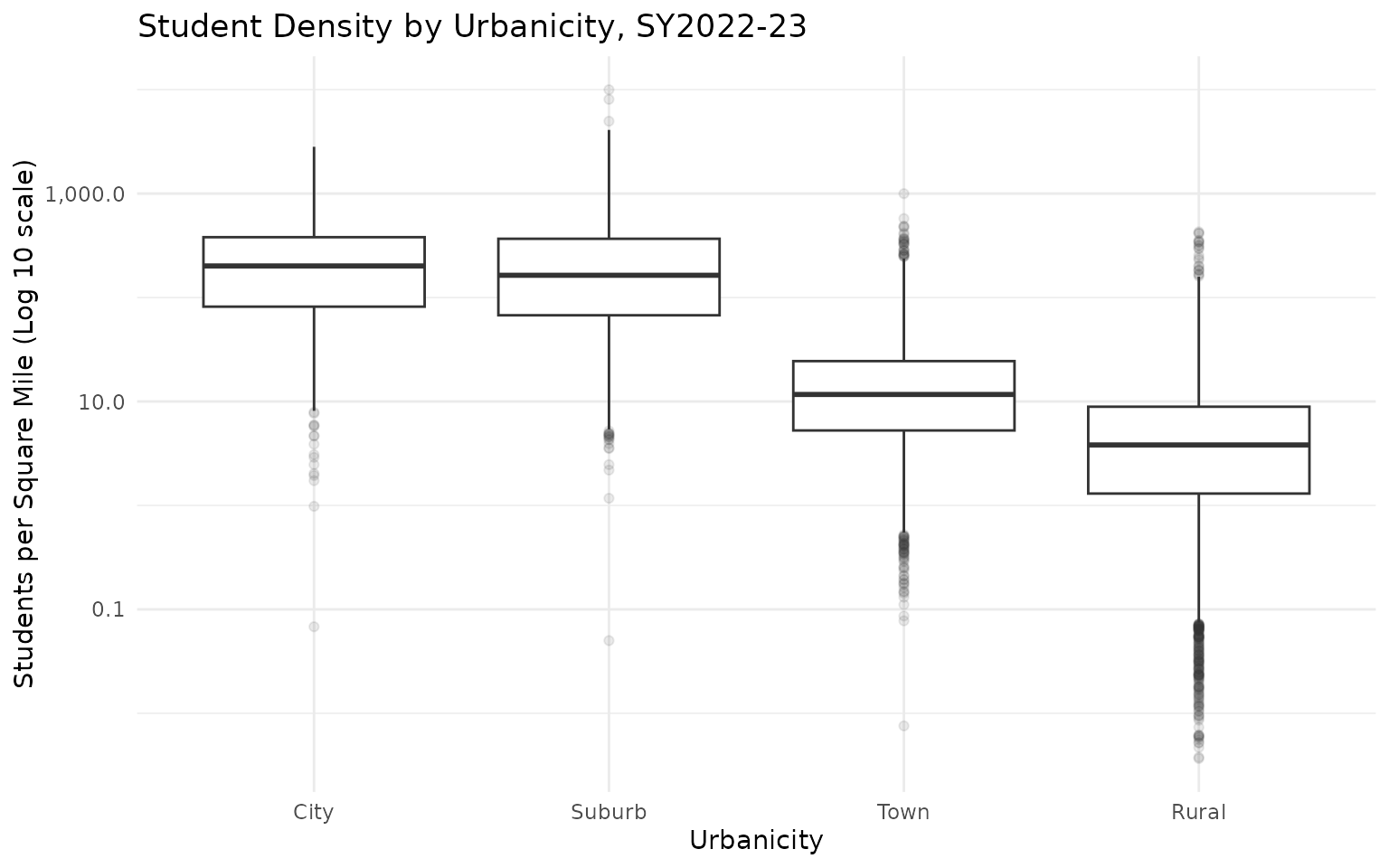
Geographic sparsity: land area and student density

urbanicity classifies districts into four categories, but districts within the same category still span a wide range of physical sparsity. s_per_sq_mi (students per square mile, derived from land_area_sq_mi) offers a continuous counterpart: a rural district serving a compact town looks different from one spread across a sparsely populated county, even though both are labeled “Rural.”

Three caveats before using it:

1. NA by design, not missingness. Districts without a Census boundary – such as charter schools – have no Gazetteer file match, so land_area_sq_mi and s_per_sq_mi are NA for them in every year.
2. NA, never Inf. Where land_area_sq_mi is zero or unavailable, s_per_sq_mi is NA rather than an infinite or undefined ratio.
3. Vermont coverage gap. Vermont’s Act 46 district consolidation left many post-consolidation LEAs without a matching Gazetteer boundary; match rates there run roughly 7-12% for those years, versus 97%+ elsewhere. Restrict Vermont density analyses to FY2012-FY2015 or FY2022 onward.

Density varies by orders of magnitude across urbanicity categories, so a log scale can be useful:

us_2023 |>
  filter(!is.na(urbanicity), !is.na(s_per_sq_mi)) |>
  ggplot(aes(x = urbanicity, y = s_per_sq_mi)) +
  geom_boxplot(outlier.alpha = 0.1) +
  scale_y_log10(labels = scales::label_comma()) +
  labs(
    title = "Student Density by Urbanicity, SY2022-23",
    x = "Urbanicity", y = "Students per Square Mile (Log 10 scale)"
  ) +
  theme_minimal()

See also

• The “Data Quality and Comparability” article, including its notes on ACS timing and panel composition.
• The “Mapping School Finance Data” article to see these measures on a map.